How to Use Image Embeddings for Object Localization
While it’s no secret that the field of object detection is making massive strides, we’ve got our eye on another rapidly advancing field: object localization. Though they sound similar, the two fields are drastically different. Object detection is about classifying what is in an image, while object localization goes one step further to identify where the objects are in the image. For example, a self-driving car might detect a dog in its view, but that is not nearly as helpful as knowing where the dog is relative to the car: Is it on the road in the vehicle’s way? Or is it safely on the sidewalk?
The abundance of research in this area has produced many open source libraries for object detection, including YOLOv3, and Facebook’s Detectron. And while using open source libraries are helpful, writing code yourself is more beneficial—especially if you want to gain a deeper understanding of how the technology works. Get ready to learn how to identify a dataset, embed images into vector space, train a localization network, and evaluate the results.
Identify a Dataset
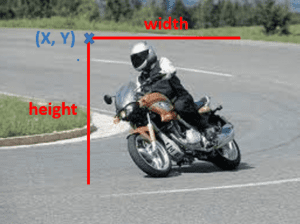
To localize objects in an image, you need to go beyond simple images with class labels as your training data. For each object, you’ll need coordinates of a bounding box (an x, y point) as well as the box’s height and width. While this makes data collection more difficult, there are some open source datasets that make it easier to get started. For this example, we use data from Pascal VOC. This particular dataset consists of images as inputs, as well as object classes and bounding box coordinates as outputs.
Project Images into Vector Space
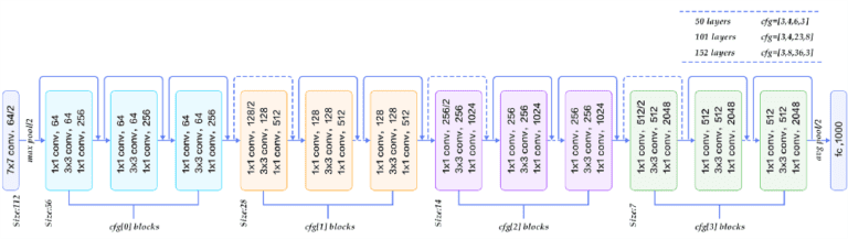
The secret sauce of deep neural networks is the rich feature engineering done in the layer before the classifier. You can think of this learned data representation as an embedding. Essentially, you learn to take an image, and represent that image as a set of numbers (vector or matrix). For this example, we generate our image embedding using ResNet50 (see Figure 2).
Figure 2: Image Courtesy of https://medium.com/@siddharthdas_32104/cnns-architectures-lenet-alexnet-vgg-googlenet-resnet-and-more-666091488df5
The model was originally trained to take an input image and predict the class of object in it—a decent surrogate for our task. We take the full pre-trained model and cut off the last few layers of the network, since we want its learned image embedding rather than its class prediction. Then we can pass all our Pascal VOC images through the chopped network to obtain a fixed length vector representation of the image. Here’s the code to grab ResNet and chop off the pooling layers:
# import the packages used

from keras.applications.resnet50 import ResNet50

from keras.models import Model


# grab the pre-trained ResNet model

resnet = ResNet50(include_top=False)


# define the input and outputs we want to use,

# note that we cut off the last 2 layers (pooling)

inp = resnet.layers[0].input

output = resnet.layers[-2].output


# define our model that computes embeddings for Pascal VOC images

embedding_model = Model(inputs=inp, outputs=output)
Train a Localizer
The input to our localization model is the learned embeddings of images and our output is both the class of the object in the image as well as the bounding box for the object. Therefore, we have 2 loss functions: categorical cross entropy for classification and mean squared error for the bounding box. In theory, you could train the network to output only the bounding box. However, knowing that the object in the image is a dog versus a differently-shaped object like a person, improves the bounding box predictions. Due to these synergies between the two tasks, you get better results using multi-task learning. The resulting network can predict what object is in an image as well as where the object is, given an input image.
Evaluate the Results
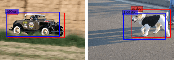
Now that our model is trained, we can do nifty things like plotting our actual bounding box and our predicted bounding box—along with actual and predicted class—on the original images (Figure 3). This exercise is useful to visually evaluate your model’s predictions. If our predictions are consistently off, our self-driving car may end up hitting more things. On the other hand, with more accurate predictions the self-driving car will be significantly safer.
Figure 3: Left image is a car with actual and predicted bounding box. Right image is a dog with actual and predicted bounding box. Red box is actual, blue box is predicted.
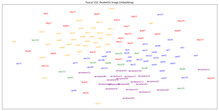
One added bonus of embedding our input images into vector space is that we can visualize them using t-SNE—an algorithm that learns to project data in high dimensional space into lower dimensional space while preserving global and local distances (see Figure 4).
Figure 4: Plot of Pascal VOC images in vector space using image embeddings from ResNet.
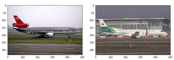
In the above plot, images close to one another tend to be more similar, whereas images far apart are less similar. For instance, the two images in Figure 5 were very close in vector space and look very similar visually.
Figure 5: Images our embeddings believed to be similar are in fact similar visually. Left: ‘aeroplane98’, Right: ‘aeroplane30’.
In the business world, techniques like this can be leveraged in creative ways to build new applications and modernize legacy ones. For example, a social media app could use object localization in a picture auto-tagging feature and a marketing agency could use image embeddings to retrieve similar images for use in copy. Want to understand how we can help you leverage these analytics? Get started with Predictive Analytics Discovery.